How to Solve Log Equations Basics

Table of Contents
- Understanding the Basics of Logarithmic Equations
- Differences between Logarithmic and Linear Equations
- Real-life Scenarios where Logarithmic Equations are Applied
- Types of Logarithmic Equations
- Exponential Equations
- Logarithmic Equations
- Properties of Logarithmic Equations
- Table of Logarithmic Equations, How to solve log equations
- Solving Logarithmic Equations with the Same Base: How To Solve Log Equations
- Properties of Logarithmic Equations with the Same Base
- Step-by-Step Solutions
- Importance of Identifying Correct Base
- Solving Logarithmic Equations with Different Bases
- Conversion Between Different Bases
- Utilizing Logarithmic Properties to Simplify Equations
- Product Rule:
- Power Rule:
- Graphical Representation of Logarithmic Equations
- Creating Graphs of Logarithmic Equations
- Characteristics of Graphs of Logarithmic Equations
- Real-World Applications of Graphical Representation of Logarithmic Equations
- Importance of Graphical Representation in Solving Logarithmic Equations
- Real-Life Examples of Graphical Representations of Logarithmic Functions
- Conclusive Thoughts
- FAQ Summary
Delving into how to solve log equations, this introduction immerses readers in a unique and compelling narrative. Logarithmic equations are a fundamental concept in mathematics, and understanding them is essential for solving various problems in science, engineering, and economics.
In this article, we will explore the basics of logarithmic equations, including the definition, properties, and applications. We will also discuss how to solve logarithmic equations with the same and different bases, and provide examples and tips for graphical representation and advanced topics.
Understanding the Basics of Logarithmic Equations
In the realm of mathematics, logarithmic equations stand as a unique breed of problems that have the power to unravel the mysteries of growth and decay. These equations are the foundation upon which many advanced mathematical concepts are built. Logarithmic equations deal with the study of numbers and their relationship to their base values in a particular mathematical operation. They provide insights into the rate at which quantities increase or decrease.
Unlike linear equations, which are as straightforward as the path a straight line takes through a graph, logarithmic equations weave a complex web of relationships between variables. In linear equations, each unit change in a variable corresponds to a proportional change in the dependent variable. However, in logarithmic equations, the relationship is non-linear – each unit change in the independent variable causes a constant percentage or proportional change in the dependent variable.
Logarithmic equations are deeply rooted in everyday life, yet the majority of people remain oblivious to their existence. Real-life applications can be observed in various fields such as finance, physics, engineering, and even medicine. In finance, logarithmic equations are used to calculate the returns on investment; in physics, they help us understand the exponential decay of radioactive materials; and in engineering, they play a crucial role in the design of electronic circuits and the prediction of population growth.
Differences between Logarithmic and Linear Equations
Logarithmic equations diverge from linear equations at a fundamental level. In linear equations, the relationship between the variables is direct and proportional, resulting in a linear graph with a constant slope. On the other hand, logarithmic equations are characterized by their non-linear nature, where the dependent variable grows at a constant rate, but not in proportion to the independent variable. This distinction between linear and logarithmic behavior can be attributed to the exponential nature of logarithmic equations.- Linear Equations The equation y = mx + b represents a linear relationship between the variables y and x, where m is the slope and b is the y-intercept. In this type of equation, each unit change in x corresponds to a proportional change in y. For example, if a car travels x miles at a speed of m miles per hour, it will take 1/x hours to cover that distance.
- Logarithmic Equations The equation y = a (x^k) represents a logarithmic relationship between the variables y and x, where a is the coefficient and k is the exponent. In this type of equation, each unit change in x causes a constant percentage or proportional change in y. For instance, if a population is growing at a rate of 10% per annum, the population after n years can be represented by the equation p(n) = p0 e^(0.10n), where p0 is the initial population and e is the base of the natural logarithm.
Real-life Scenarios where Logarithmic Equations are Applied
Logarithmic equations have a broad spectrum of applications in various fields of study and engineering practices. In the field of finance, logarithmic equations are used to calculate the returns on investment, where the change in investment value over time is modeled using an exponential function. The formula to calculate the return on investment (ROI) is given by: ROI = (final value/initial value)^1/n - 1."A logarithmic function is a mathematical function that models exponential or power-law growth or decay. Logarithmic functions and exponential functions are inverses of each other." — Source
| Example | Description |
|---|---|
| Population Growth | The growth of a population can be modeled using logarithmic equations, where the population size at any given time is directly proportional to the amount of time elapsed. For example, if a population is growing at a rate of 3% per annum, the population after n years can be represented by the equation p(n) = p0 (1 + 0.03)^n. |
| Radioactive Decay | Radioactive decay is an example of an exponential decay process, which can be modeled using logarithmic equations. The formula to calculate the amount of a radioactive substance remaining after n time units is given by: N(t) = N0 e^(-k t), where N0 is the initial amount, e is the base of the natural logarithm, and k is the decay constant. |
| Compound Interest | Compound interest is a type of interest that is calculated on both the initial investment and any accrued interest. The formula to calculate the future value of an investment with compound interest is given by: A = P (1 + r/n)^(n*t), where A is the amount, P is the principal, r is the interest rate, n is the number of times interest is compounded per year, and t is the time in years. |
Types of Logarithmic Equations
Exponential Equations
Exponential equations are in the form ofy = b^x, where 'b' is the base and 'x' is the exponent. These equations represent exponential growth or decay, where the logarithmic form is the inverse. For instance, the equation
2^3 = 8is an exponential equation, where the base 'b' is 2 and the exponent 'x' is 3. To convert this to a logarithmic equation, we take the logarithm of both sides.
Logarithmic Equations
Logarithmic equations, on the other hand, are in the form oflogb(x) = y, where 'b' is the base and 'x' is the argument. These equations represent the inverse operation of exponential equations. For instance, the equation
log2(8) = 3is a logarithmic equation, where the base 'b' is 2 and the argument 'x' is 8.
Properties of Logarithmic Equations
The properties of logarithmic equations include:- The product property:
logb(xy) = logb(x) + logb(y)
- The power property:
logb(x^y) = y logb(x)
- The quotient property:
logb(x/y) = logb(x) - logb(y)
- The reciprocal property:
logb(1/x) = -logb(x)
Table of Logarithmic Equations, How to solve log equations
| Equation Type | Formula | Description || --- | --- | --- |
| Exponential | y = b^x | Exponential growth or decay |
| Logarithmic | logb(x) = y | Inverse operation of exponential equation |
| Product Property | logb(xy) = logb(x) + logb(y) | Logarithm of product is sum of logs |
| Power Property | logb(x^y) = y logb(x) | Logarithm of power is exponent times log |
| Quotient Property | logb(x/y) = logb(x) - logb(y) | Logarithm of quotient is log of numerator minus log of denominator |
| Reciprocal Property | logb(1/x) = -logb(x) | Logarithm of reciprocal is negative log |
Solving Logarithmic Equations with the Same Base: How To Solve Log Equations
Properties of Logarithmic Equations with the Same Base
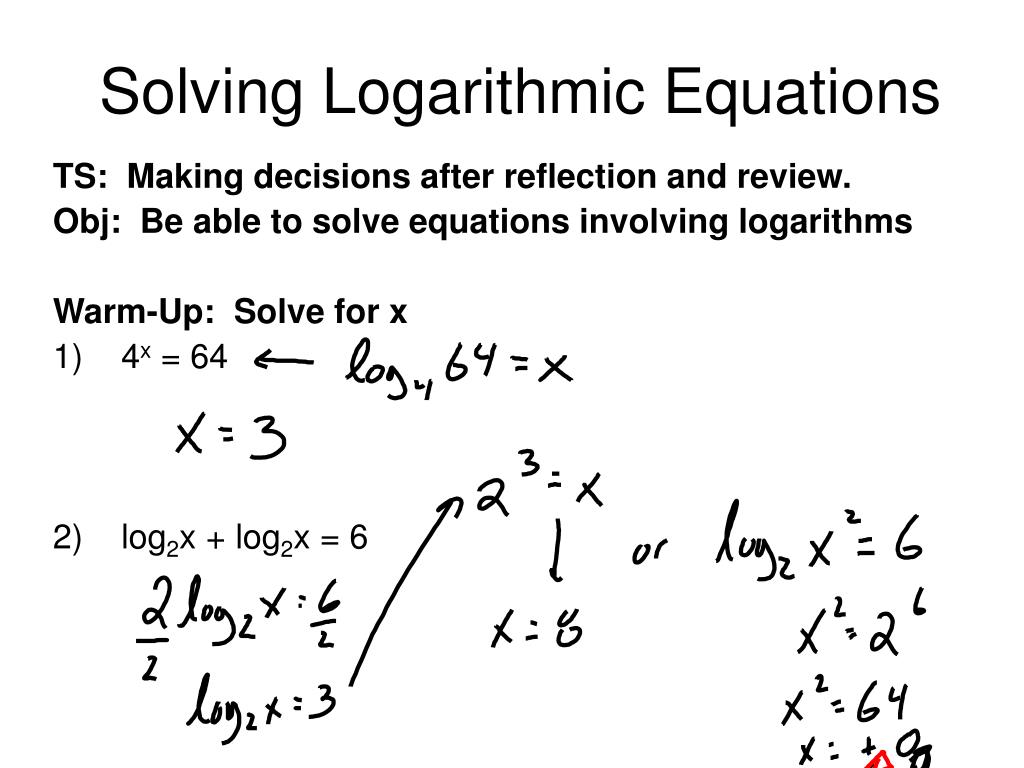
When dealing with logarithmic equations that have the same base, we can utilize various properties to simplify and solve them. One fundamental property is the one-to-one correspondence between logarithmic and exponential functions. This means that if loga(x) = y, then a^y = x. By leveraging this property, we can rewrite the logarithmic equation in a form that is easier to solve.Step-by-Step Solutions
Example 1: Solving a Logarithmic Equation with the Same BaseWe are given the equation log2(x) = 4. We need to solve for x.
* Step 1: Rewrite the logarithmic equation using the one-to-one correspondence property. This gives us 2^4 = x.
Example 2: Solving a Logarithmic Equation with the Same Base We are given the equation log5(x) = 3. We need to solve for x.
* Step 1: Rewrite the logarithmic equation using the one-to-one correspondence property. This gives us 5^3 = x.
Importance of Identifying Correct Base
Identifying the correct base is a crucial step when solving logarithmic equations. If the base is incorrect, the entire solution will be incorrect. This can lead to a multitude of problems, including incorrect conclusions, flawed reasoning, and even wrong answers.Common Mistakes to Avoid
When dealing with logarithmic equations, some common mistakes to avoid include:
* Incorrectly identifying the base
By being aware of these common pitfalls and taking the time to carefully analyze the equation, we can ensure that our solutions are accurate and reliable.
Solving Logarithmic Equations with Different Bases
Conversion Between Different Bases
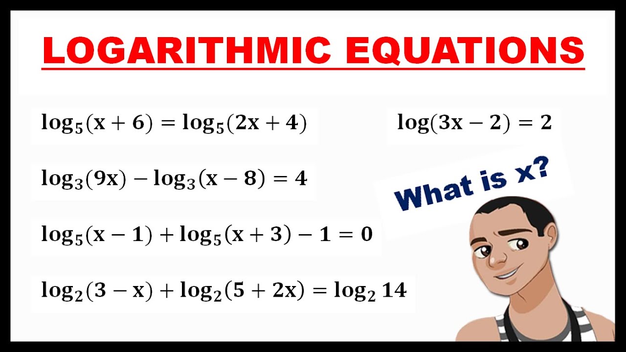
Converting between different bases is a crucial step in solving logarithmic equations. The propertylog_b(y) = (log_a(y)) / (log_a(b))allows us to express a logarithm with one base in terms of another base. This property is derived from the change-of-base formula, which states
log_b(y) = log_k(y) / log_k(b)where k is an arbitrary base.
Utilizing Logarithmic Properties to Simplify Equations
When confronted with logarithmic equations featuring different bases, the key is to recognize and apply relevant logarithmic properties. The product rule, quotient rule, and power rule can be used to simplify and manipulate logarithmic expressions, facilitating the solution of equations with varying bases. These rules are summarized as follows:Product Rule:
If log_b(y) = x, then log_b(y) + log_b(z) = x + log_b(z)- log_b(yz) = log_b(y) + log_b(z)
- log_b(y/z) = log_b(y) - log_b(z)
Power Rule:
If log_b(y) = x, then log_b(y^n) = n log_b(y)- log_b(y^n) = n log_b(y)
- log_b(y^(m/n)) = (m/n) log_b(y)
Graphical Representation of Logarithmic Equations
The graphical representation of logarithmic equations is a powerful tool in understanding the behavior and properties of logarithmic functions. By plotting the graph of a logarithmic equation, we can visualize its key characteristics, such as its domain and range, x-intercepts, and vertical asymptotes.Creating Graphs of Logarithmic Equations
To create a graph of a logarithmic equation, we can use various graphing methods, including the use of a graphing calculator or software. For example, we can plot the graph of the function f(x) = log(x) + 3, where log(x) denotes the natural logarithm of x. To do this, we can first determine the domain of the function, which is all real numbers greater than 0. We can then plot a few points on the graph, such as (1, 3), (10, 4), and (100, 5), and join the points with a smooth curve.Characteristics of Graphs of Logarithmic Equations
The graph of a logarithmic equation typically exhibits several key characteristics, including a vertical asymptote at x = 0, a horizontal asymptote at y = constant, and a smooth curve that increases or decreases as x increases. The graph may also have x-intercepts or zeros, which correspond to values of x for which the function equals zero.- Vertical Asymptote at x = 0 The graph of a logarithmic equation typically has a vertical asymptote at x = 0, which means that the function becomes increasingly large as x approaches 0. This can be seen in the graph of f(x) = log(x + 1), where the graph approaches infinity as x approaches 0.
- Horizontal Asymptote at y = Constant The graph of a logarithmic equation may also have a horizontal asymptote at y = constant, which means that the function approaches a constant value as x approaches infinity. This can be seen in the graph of f(x) = log(x), where the graph approaches infinity as x approaches infinity.
- X-Intercepts or Zeros The graph of a logarithmic equation may also have x-intercepts or zeros, which correspond to values of x for which the function equals zero. For example, the graph of f(x) = log(x - 1) has an x-intercept at x = 1.
The graph of a logarithmic equation is a powerful tool in understanding its behavior and properties.
Real-World Applications of Graphical Representation of Logarithmic Equations
The graphical representation of logarithmic equations has many real-world applications, including modeling population growth, measuring sound levels, and calculating pH levels. For example, the graph of f(x) = log2(x) + 3 can be used to model the growth of a population of microorganisms, where x represents the time in days and f(x) represents the population size.The graphical representation of logarithmic equations is a powerful tool in understanding and applying logarithmic functions in real-world situations.
Importance of Graphical Representation in Solving Logarithmic Equations
The graphical representation of logarithmic equations is an important tool in solving logarithmic equations, as it allows us to visualize the behavior of the function and make informed decisions about the solution. By plotting the graph of a logarithmic equation, we can identify the domain and range of the function, the location of x-intercepts and vertical asymptotes, and other key characteristics that can aid in solving the equation.Real-Life Examples of Graphical Representations of Logarithmic Functions
Here are a few real-life examples of graphical representations of logarithmic functions:- Modeling Population Growth The graph of f(x) = log2(x) + 3 can be used to model the growth of a population of microorganisms, where x represents the time in days and f(x) represents the population size.
- Measuring Sound Levels The graph of f(x) = log10(x) + 5 can be used to measure sound levels, where x represents the decibel level and f(x) represents the corresponding sound pressure level.
- Calculating pH Levels The graph of f(x) = log10(x) + 7 can be used to calculate pH levels, where x represents the concentration of hydrogen ions and f(x) represents the corresponding pH value.
Conclusive Thoughts
Understanding how to solve log equations is a crucial skill that can be applied in various fields. By following the tips and techniques Artikeld in this article, readers can improve their problem-solving skills and become proficient in working with logarithmic equations.
Whether you are a student or a professional, this article aims to provide a comprehensive guide on how to solve log equations, making it a valuable resource for anyone looking to expand their mathematical knowledge.
FAQ Summary
Q: What is the difference between a logarithmic equation and a linear equation?
A: A logarithmic equation is an equation in which the variable appears as the logarithm of an expression, whereas a linear equation is an equation in which the variable appears as a coefficient or an exponent.
Q: How do I choose the correct base when solving logarithmic equations?
A: The correct base should be chosen based on the given problem and the context. If the problem involves a natural logarithm, the base is typically e. If the problem involves a common logarithm, the base is typically 10.
Q: Can logarithmic equations be simplified?
A: Yes, logarithmic equations can be simplified using logarithmic properties such as the product property and the power property.
Q: How do I determine the domain and range of a logarithmic function?
A: The domain of a logarithmic function is defined as the set of all real numbers greater than zero, and the range is defined as the set of all real numbers.
Q: Can logarithmic equations be graphed?
A: Yes, logarithmic equations can be graphed using a graphing calculator or software. The graph of a logarithmic function has a vertical asymptote at x = 0, and the function approaches infinity as x approaches positive infinity.
Q: What are some real-world applications of logarithmic equations?
A: Logarithmic equations have many real-world applications, including population growth, compound interest calculations, and sound level measurements.
Leave a Comment
Comments are moderated before appearing. The data you submit is processed according to the Privacy Policy of blog.poolsupplies.com.